library(tidyverse)
penguins <- palmerpenguins::penguins |>
  filter(!is.na(sex))
penguins
## # A tibble: 333 × 8
##    species island    bill_length_mm bill_depth_mm flipper_length_mm body_mass_g
##    <fct>   <fct>              <dbl>         <dbl>             <int>       <int>
##  1 Adelie  Torgersen           39.1          18.7               181        3750
##  2 Adelie  Torgersen           39.5          17.4               186        3800
##  3 Adelie  Torgersen           40.3          18                 195        3250
##  4 Adelie  Torgersen           36.7          19.3               193        3450
##  5 Adelie  Torgersen           39.3          20.6               190        3650
##  6 Adelie  Torgersen           38.9          17.8               181        3625
##  7 Adelie  Torgersen           39.2          19.6               195        4675
##  8 Adelie  Torgersen           41.1          17.6               182        3200
##  9 Adelie  Torgersen           38.6          21.2               191        3800
## 10 Adelie  Torgersen           34.6          21.1               198        4400
## # ℹ 323 more rows
## # ℹ 2 more variables: sex <fct>, year <int>1 Getting started
In this chapter, we’re going to do two things:
- Learn simple guidelines for better tables
- Implement them with
{gt}
And of course we will need data for that. I like penguins, so we’re going to use the fabulous penguins data set from {palmerpenguins}.
Using this data, let us count the penguins. These counts will serve as a simple data set to practice table building.
penguin_counts <- penguins |>
  mutate(year = as.character(year)) |>
  group_by(species, island, sex, year) |>
  summarise(n = n(), .groups = 'drop')
penguin_counts
## # A tibble: 30 × 5
##    species island sex    year      n
##    <fct>   <fct>  <fct>  <chr> <int>
##  1 Adelie  Biscoe female 2007      5
##  2 Adelie  Biscoe female 2008      9
##  3 Adelie  Biscoe female 2009      8
##  4 Adelie  Biscoe male   2007      5
##  5 Adelie  Biscoe male   2008      9
##  6 Adelie  Biscoe male   2009      8
##  7 Adelie  Dream  female 2007      9
##  8 Adelie  Dream  female 2008      8
##  9 Adelie  Dream  female 2009     10
## 10 Adelie  Dream  male   2007     10
## # ℹ 20 more rows
In an actual table, the data would probably be rearranged a bit. There’s nothing wrong with this long (i.e. many rows) data format. In fact, this format is great for data analysis. But in a table that is meant to be read by humans, not machines, you’ll probably go with a wider format.
penguin_counts_wider <- penguin_counts |>
  pivot_wider(
    names_from = c(species, sex),
    values_from = n
  ) |>
  # Make missing numbers (NAs) into zero
  mutate(across(.cols = -(1:2), .fns = ~replace_na(., replace = 0))) |>
  arrange(island, year)
penguin_counts_wider
## # A tibble: 9 × 8
##   island    year  Adelie_female Adelie_male Chinstrap_female Chinstrap_male
##   <fct>     <chr>         <int>       <int>            <int>          <int>
## 1 Biscoe    2007              5           5                0              0
## 2 Biscoe    2008              9           9                0              0
## 3 Biscoe    2009              8           8                0              0
## 4 Dream     2007              9          10               13             13
## 5 Dream     2008              8           8                9              9
## 6 Dream     2009             10          10               12             12
## 7 Torgersen 2007              8           7                0              0
## 8 Torgersen 2008              8           8                0              0
## 9 Torgersen 2009              8           8                0              0
## # ℹ 2 more variables: Gentoo_female <int>, Gentoo_male <int>
Now, let’s put this into a table. Not too long ago I would have probably visualized the data with a table like this:
penguins_counts_wider data set created by yours truly with LibreOffice Calc (spreadsheet software - double ugh. Though, compared to Excel it’s open-source. So maybe 1.5 ugh?)
Ugh. This is not a sexy table. I get bored just looking at that. So let’s improve this table. To do so, here are the 6 guidelines that will, well, guide us.
- Avoid vertical lines
- Use better column names
- Align columns
- Use groups instead of repetitive columns
- Remove missing numbers
- Add summaries
1.1 Avoid vertical lines
This is the guideline that gives you the biggest bang for your buck. The above table uses waaaay to many grid lines. Without vertical lines, the table will look less cramped.
Thankfully, {gt} seems to live by this rule as it is implemented by default. Thus, we only need to pass our data set penguin_counts_wider to gt(). You can think of this function as the ggplot() analogue: It’s the starting point of any table in the {gt} universe.
library(gt)
penguin_counts_wider |>
gt() | island | year | Adelie_female | Adelie_male | Chinstrap_female | Chinstrap_male | Gentoo_female | Gentoo_male |
|---|---|---|---|---|---|---|---|
| Biscoe | 2007 | 5 | 5 | 0 | 0 | 16 | 17 |
| Biscoe | 2008 | 9 | 9 | 0 | 0 | 22 | 23 |
| Biscoe | 2009 | 8 | 8 | 0 | 0 | 20 | 21 |
| Dream | 2007 | 9 | 10 | 13 | 13 | 0 | 0 |
| Dream | 2008 | 8 | 8 | 9 | 9 | 0 | 0 |
| Dream | 2009 | 10 | 10 | 12 | 12 | 0 | 0 |
| Torgersen | 2007 | 8 | 7 | 0 | 0 | 0 | 0 |
| Torgersen | 2008 | 8 | 8 | 0 | 0 | 0 | 0 |
| Torgersen | 2009 | 8 | 8 | 0 | 0 | 0 | 0 |
This isn’t a great table yet but it’s a start. In any case, it feels more open due to less grid lines. Of course, the column labels could be better which brings us to our next point.
1.2 Use better column names
To change the column names use the “layer” called cols_layer(). Much like {ggplot2}, {gt} works with layers. To change anything about the table, we just pass the table from layer to the next. This works with piping. Armed with that knowledge, we could label the columns like we did in Figure 1.1.
penguin_counts_wider |>
  gt() |>
  cols_label(
    island = 'Island',
    year = 'Year',
    Adelie_female = 'Adelie (female)',
    Adelie_male = 'Adelie (male)',
    Chinstrap_female = 'Chinstrap (female)',
    Chinstrap_male = 'Chinstrap (male)',
    Gentoo_female = 'Gentoo (female)',
    Gentoo_male = 'Gentoo (male)',
)| Island | Year | Adelie (female) | Adelie (male) | Chinstrap (female) | Chinstrap (male) | Gentoo (female) | Gentoo (male) |
|---|---|---|---|---|---|---|---|
| Biscoe | 2007 | 5 | 5 | 0 | 0 | 16 | 17 |
| Biscoe | 2008 | 9 | 9 | 0 | 0 | 22 | 23 |
| Biscoe | 2009 | 8 | 8 | 0 | 0 | 20 | 21 |
| Dream | 2007 | 9 | 10 | 13 | 13 | 0 | 0 |
| Dream | 2008 | 8 | 8 | 9 | 9 | 0 | 0 |
| Dream | 2009 | 10 | 10 | 12 | 12 | 0 | 0 |
| Torgersen | 2007 | 8 | 7 | 0 | 0 | 0 | 0 |
| Torgersen | 2008 | 8 | 8 | 0 | 0 | 0 | 0 |
| Torgersen | 2009 | 8 | 8 | 0 | 0 | 0 | 0 |
But this isn’t a great way to label the columns. So let’s do something else instead. First, let us create so-called spanners. These are joined columns and can be created with tab_spanner() layers. You’ll need one layer for each spanner.
penguin_counts_wider |>
  gt() |>
  cols_label(
    island = 'Island',
    year = 'Year',
    Adelie_female = 'Adelie (female)',
    Adelie_male = 'Adelie (male)',
    Chinstrap_female = 'Chinstrap (female)',
    Chinstrap_male = 'Chinstrap (male)',
    Gentoo_female = 'Gentoo (female)',
    Gentoo_male = 'Gentoo (male)',
  ) |>
  tab_spanner(
    label = md('**Adelie**'),
    columns = 3:4
  ) |>
  tab_spanner(
    label = md('**Chinstrap**'),
    columns = c('Chinstrap_female', 'Chinstrap_male')
  ) |>
  tab_spanner(
    label =  md('**Gentoo**'),
    columns = contains('Gentoo')
)| Island | Year |
Adelie
|
Chinstrap
|
Gentoo
|
|||
|---|---|---|---|---|---|---|---|
| Adelie (female) | Adelie (male) | Chinstrap (female) | Chinstrap (male) | Gentoo (female) | Gentoo (male) | ||
| Biscoe | 2007 | 5 | 5 | 0 | 0 | 16 | 17 |
| Biscoe | 2008 | 9 | 9 | 0 | 0 | 22 | 23 |
| Biscoe | 2009 | 8 | 8 | 0 | 0 | 20 | 21 |
| Dream | 2007 | 9 | 10 | 13 | 13 | 0 | 0 |
| Dream | 2008 | 8 | 8 | 9 | 9 | 0 | 0 |
| Dream | 2009 | 10 | 10 | 12 | 12 | 0 | 0 |
| Torgersen | 2007 | 8 | 7 | 0 | 0 | 0 | 0 |
| Torgersen | 2008 | 8 | 8 | 0 | 0 | 0 | 0 |
| Torgersen | 2009 | 8 | 8 | 0 | 0 | 0 | 0 |
As you can see, tab_spanner() always requires two arguments label and columns. For the columns argument I have shown you three ways to get the job done:
- Vector of column numbers
- Vector of column names
- tidyselect helpers
For the label argument you can either just state a character vector or you can wrap one in md() to enable Markdown syntax (like **bold text**).
Okay, now we don’t really need the Species labels in the actual column names anymore. The spanners already state that for us. So, let us modify our previous code to rename the columns. To do so, let me show you a cool trick that may save you some tedious typing.
First, we create a named vector that contains the actual and the desired column names.
actual_colnames <- colnames(penguin_counts_wider)
actual_colnames
## [1] "island"           "year"             "Adelie_female"    "Adelie_male"
## [5] "Chinstrap_female" "Chinstrap_male"   "Gentoo_female"    "Gentoo_male"
desired_colnames <- actual_colnames |>
  str_remove('(Adelie|Gentoo|Chinstrap)_') |>
  str_to_title()

names(desired_colnames) <- actual_colnames
desired_colnames
##           island             year    Adelie_female      Adelie_male
##         "Island"           "Year"         "Female"           "Male"
## Chinstrap_female   Chinstrap_male    Gentoo_female      Gentoo_male
##         "Female"           "Male"         "Female"           "Male"
Then, we can use this named vector as the .list argument in cols_label().
penguin_counts_wider |>
  gt() |>
  cols_label(.list = desired_colnames) |>
  tab_spanner(
    label = md('**Adelie**'),
    columns = 3:4
  ) |>
  tab_spanner(
    label = md('**Chinstrap**'),
    columns = c('Chinstrap_female', 'Chinstrap_male')
  ) |>
  tab_spanner(
    label =  md('**Gentoo**'),
    columns = contains('Gentoo')
)| Island | Year |
Adelie
|
Chinstrap
|
Gentoo
|
|||
|---|---|---|---|---|---|---|---|
| Female | Male | Female | Male | Female | Male | ||
| Biscoe | 2007 | 5 | 5 | 0 | 0 | 16 | 17 |
| Biscoe | 2008 | 9 | 9 | 0 | 0 | 22 | 23 |
| Biscoe | 2009 | 8 | 8 | 0 | 0 | 20 | 21 |
| Dream | 2007 | 9 | 10 | 13 | 13 | 0 | 0 |
| Dream | 2008 | 8 | 8 | 9 | 9 | 0 | 0 |
| Dream | 2009 | 10 | 10 | 12 | 12 | 0 | 0 |
| Torgersen | 2007 | 8 | 7 | 0 | 0 | 0 | 0 |
| Torgersen | 2008 | 8 | 8 | 0 | 0 | 0 | 0 |
| Torgersen | 2009 | 8 | 8 | 0 | 0 | 0 | 0 |
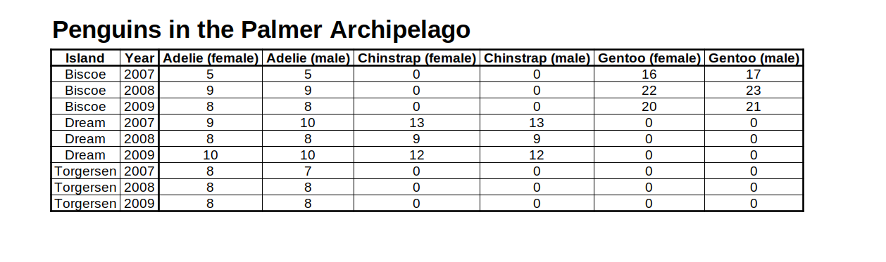
Finally, while we’re currently changing labels, let us add one important label - the title. The tab_header() layer does the trick.
penguin_counts_wider |>
  gt() |>
  cols_label(.list = desired_colnames) |>
  tab_spanner(
    label = md('**Adelie**'),
    columns = 3:4
  ) |>
  tab_spanner(
    label = md('**Chinstrap**'),
    columns = c('Chinstrap_female', 'Chinstrap_male')
  ) |>
  tab_spanner(
    label =  md('**Gentoo**'),
    columns = contains('Gentoo')
  ) |>
  tab_header(
    title = 'Penguins in the Palmer Archipelago',
    subtitle = 'Data is courtesy of the {palmerpenguins} R package'
) | Penguins in the Palmer Archipelago | |||||||
| Data is courtesy of the {palmerpenguins} R package | |||||||
| Island | Year |
Adelie
|
Chinstrap
|
Gentoo
|
|||
|---|---|---|---|---|---|---|---|
| Female | Male | Female | Male | Female | Male | ||
| Biscoe | 2007 | 5 | 5 | 0 | 0 | 16 | 17 |
| Biscoe | 2008 | 9 | 9 | 0 | 0 | 22 | 23 |
| Biscoe | 2009 | 8 | 8 | 0 | 0 | 20 | 21 |
| Dream | 2007 | 9 | 10 | 13 | 13 | 0 | 0 |
| Dream | 2008 | 8 | 8 | 9 | 9 | 0 | 0 |
| Dream | 2009 | 10 | 10 | 12 | 12 | 0 | 0 |
| Torgersen | 2007 | 8 | 7 | 0 | 0 | 0 | 0 |
| Torgersen | 2008 | 8 | 8 | 0 | 0 | 0 | 0 |
| Torgersen | 2009 | 8 | 8 | 0 | 0 | 0 | 0 |
By the same trick we could also add a caption for a Quarto document (tab_caption()), a footnote (tab_footnote()) or another source note (tab_sourcenote()), In this case it’s a bit much, though. So I won’t add them. Just know that these functions exist in case you need them. For now, let us talk about our next guideline.
Before we can do that, let me mention one small thing: Our spanners and headers will not change as we move along this tutorial. To avoid repeating them all the time, let me wrap them in a function.
spanners_and_header <- function(gt_tbl) {
  gt_tbl |>
    tab_spanner(
      label = md('**Adelie**'),
      columns = 3:4
    ) |>
    tab_spanner(
      label = md('**Chinstrap**'),
      columns = c('Chinstrap_female', 'Chinstrap_male')
    ) |>
    tab_spanner(
      label =  md('**Gentoo**'),
      columns = contains('Gentoo')
    ) |>
    tab_header(
      title = 'Penguins in the Palmer Archipelago',
      subtitle = 'Data is courtesy of the {palmerpenguins} R package'
    )
}

# This produces the same output
penguin_counts_wider |>
  gt() |>
  cols_label(.list = desired_colnames)  |>
spanners_and_header() | Penguins in the Palmer Archipelago | |||||||
| Data is courtesy of the {palmerpenguins} R package | |||||||
| Island | Year |
Adelie
|
Chinstrap
|
Gentoo
|
|||
|---|---|---|---|---|---|---|---|
| Female | Male | Female | Male | Female | Male | ||
| Biscoe | 2007 | 5 | 5 | 0 | 0 | 16 | 17 |
| Biscoe | 2008 | 9 | 9 | 0 | 0 | 22 | 23 |
| Biscoe | 2009 | 8 | 8 | 0 | 0 | 20 | 21 |
| Dream | 2007 | 9 | 10 | 13 | 13 | 0 | 0 |
| Dream | 2008 | 8 | 8 | 9 | 9 | 0 | 0 |
| Dream | 2009 | 10 | 10 | 12 | 12 | 0 | 0 |
| Torgersen | 2007 | 8 | 7 | 0 | 0 | 0 | 0 |
| Torgersen | 2008 | 8 | 8 | 0 | 0 | 0 | 0 |
| Torgersen | 2009 | 8 | 8 | 0 | 0 | 0 | 0 |
1.3 Align columns
Did you notice that gt() aligned the columns differently? That’s because the columns of the corresponding data.frame/tibble contained different data types. Specifically:
the counts are
integersand aligned to the rightthe
yearcolumn is acharactervector and uses alignment to the left (though it’s not totally visible because the column is narrow)the
islandcolumn is afactorand uses center alignment (even though its entries arecharacters)
It’s a good default to align numbers to the right and texts to the left. Why? Because it’s more readable. Need an example? Here’s one. Most (western) people will probably say that the left column is the easiest to read because we read from left to right.

For numbers it’s the other way around. That’s because right-aligned numbers make it easy to see how many digits a number has compared to other numbers. This assumes that your numbers use a font that assigns equal width to all digits (monospace fonts).
So, let us align the island and year column. We can either do this by transforming the data types before even calling gt(). Or we use the cols_align() layer. Once again, this layer understands text locations and tidyselection helpers.
penguin_counts_wider |>
  mutate(
    island = as.character(island),
    year = as.numeric(year)
  ) |>
  gt() |>
  cols_label(.list = desired_colnames) |>
spanners_and_header() | Penguins in the Palmer Archipelago | |||||||
| Data is courtesy of the {palmerpenguins} R package | |||||||
| Island | Year |
Adelie
|
Chinstrap
|
Gentoo
|
|||
|---|---|---|---|---|---|---|---|
| Female | Male | Female | Male | Female | Male | ||
| Biscoe | 2007 | 5 | 5 | 0 | 0 | 16 | 17 |
| Biscoe | 2008 | 9 | 9 | 0 | 0 | 22 | 23 |
| Biscoe | 2009 | 8 | 8 | 0 | 0 | 20 | 21 |
| Dream | 2007 | 9 | 10 | 13 | 13 | 0 | 0 |
| Dream | 2008 | 8 | 8 | 9 | 9 | 0 | 0 |
| Dream | 2009 | 10 | 10 | 12 | 12 | 0 | 0 |
| Torgersen | 2007 | 8 | 7 | 0 | 0 | 0 | 0 |
| Torgersen | 2008 | 8 | 8 | 0 | 0 | 0 | 0 |
| Torgersen | 2009 | 8 | 8 | 0 | 0 | 0 | 0 |
penguin_counts_wider |>
  gt() |>
  cols_label(.list = desired_colnames) |>
  spanners_and_header()  |>
  cols_align(align = 'right', columns = 'year') |>
  cols_align(
    align = 'left',
    columns = where(is.factor)
)| Penguins in the Palmer Archipelago | |||||||
| Data is courtesy of the {palmerpenguins} R package | |||||||
| Island | Year |
Adelie
|
Chinstrap
|
Gentoo
|
|||
|---|---|---|---|---|---|---|---|
| Female | Male | Female | Male | Female | Male | ||
| Biscoe | 2007 | 5 | 5 | 0 | 0 | 16 | 17 |
| Biscoe | 2008 | 9 | 9 | 0 | 0 | 22 | 23 |
| Biscoe | 2009 | 8 | 8 | 0 | 0 | 20 | 21 |
| Dream | 2007 | 9 | 10 | 13 | 13 | 0 | 0 |
| Dream | 2008 | 8 | 8 | 9 | 9 | 0 | 0 |
| Dream | 2009 | 10 | 10 | 12 | 12 | 0 | 0 |
| Torgersen | 2007 | 8 | 7 | 0 | 0 | 0 | 0 |
| Torgersen | 2008 | 8 | 8 | 0 | 0 | 0 | 0 |
| Torgersen | 2009 | 8 | 8 | 0 | 0 | 0 | 0 |
1.4 Use groups instead of repetitive columns
The island column is somewhat repetitive. In cases like these, I’d rather remove the column. Instead, I would group the table using additional rows. I like to think that this comes with better readability.
With {gt}, this grouping is easy. We only need to specify the groupname_col argument in gt(). If we want, we can also set the rowname_col argument to year. This will format the “Year” column a bit differently.
penguin_counts_wider |>
  mutate(
    island = as.character(island),
    year = as.numeric(year)
  ) |>
  gt(groupname_col = 'island') |>
  cols_label(.list = desired_colnames) |>
spanners_and_header() | Penguins in the Palmer Archipelago | ||||||
| Data is courtesy of the {palmerpenguins} R package | ||||||
| Year |
Adelie
|
Chinstrap
|
Gentoo
|
|||
|---|---|---|---|---|---|---|
| Female | Male | Female | Male | Female | Male | |
| Biscoe | ||||||
| 2007 | 5 | 5 | 0 | 0 | 16 | 17 |
| 2008 | 9 | 9 | 0 | 0 | 22 | 23 |
| 2009 | 8 | 8 | 0 | 0 | 20 | 21 |
| Dream | ||||||
| 2007 | 9 | 10 | 13 | 13 | 0 | 0 |
| 2008 | 8 | 8 | 9 | 9 | 0 | 0 |
| 2009 | 10 | 10 | 12 | 12 | 0 | 0 |
| Torgersen | ||||||
| 2007 | 8 | 7 | 0 | 0 | 0 | 0 |
| 2008 | 8 | 8 | 0 | 0 | 0 | 0 |
| 2009 | 8 | 8 | 0 | 0 | 0 | 0 |
penguin_counts_wider |>
  mutate(
    island = as.character(island),
    year = as.numeric(year)
  ) |>
  gt(groupname_col = 'island', rowname_col = 'year') |>
  cols_label(.list = desired_colnames) |>
spanners_and_header() | Penguins in the Palmer Archipelago | ||||||
| Data is courtesy of the {palmerpenguins} R package | ||||||
|
Adelie
|
Chinstrap
|
Gentoo
|
||||
|---|---|---|---|---|---|---|
| Female | Male | Female | Male | Female | Male | |
| Biscoe | ||||||
| 2007 | 5 | 5 | 0 | 0 | 16 | 17 |
| 2008 | 9 | 9 | 0 | 0 | 22 | 23 |
| 2009 | 8 | 8 | 0 | 0 | 20 | 21 |
| Dream | ||||||
| 2007 | 9 | 10 | 13 | 13 | 0 | 0 |
| 2008 | 8 | 8 | 9 | 9 | 0 | 0 |
| 2009 | 10 | 10 | 12 | 12 | 0 | 0 |
| Torgersen | ||||||
| 2007 | 8 | 7 | 0 | 0 | 0 | 0 |
| 2008 | 8 | 8 | 0 | 0 | 0 | 0 |
| 2009 | 8 | 8 | 0 | 0 | 0 | 0 |
In this case, I prefer the latter style because we don’t really need a “Year” label to identify 2007, 2008 and 2009 as years. But an island label could be nice (I’m really bad with geography). The easiest way to add that to the group names is via string manipulation before gt() is called.
penguin_counts_wider |>
  mutate(
    island = as.character(island),
    year = as.numeric(year),
    island = paste0('Island: ', island)
  ) |>
  gt(groupname_col = 'island', rowname_col = 'year') |>
  cols_label(.list = desired_colnames) |>
spanners_and_header() | Penguins in the Palmer Archipelago | ||||||
| Data is courtesy of the {palmerpenguins} R package | ||||||
|
Adelie
|
Chinstrap
|
Gentoo
|
||||
|---|---|---|---|---|---|---|
| Female | Male | Female | Male | Female | Male | |
| Island: Biscoe | ||||||
| 2007 | 5 | 5 | 0 | 0 | 16 | 17 |
| 2008 | 9 | 9 | 0 | 0 | 22 | 23 |
| 2009 | 8 | 8 | 0 | 0 | 20 | 21 |
| Island: Dream | ||||||
| 2007 | 9 | 10 | 13 | 13 | 0 | 0 |
| 2008 | 8 | 8 | 9 | 9 | 0 | 0 |
| 2009 | 10 | 10 | 12 | 12 | 0 | 0 |
| Island: Torgersen | ||||||
| 2007 | 8 | 7 | 0 | 0 | 0 | 0 |
| 2008 | 8 | 8 | 0 | 0 | 0 | 0 |
| 2009 | 8 | 8 | 0 | 0 | 0 | 0 |
1.5 Remove missing numbers
Notice that our table has a lot of zeroes in it. For better readability, let us replace the zeroes with something more lightweight. We accomplish this with the sub_zero() layer.
penguin_counts_wider |>
  mutate(
    island = as.character(island),
    year = as.numeric(year),
    island = paste0('Island: ', island)
  ) |>
  gt(groupname_col = 'island', rowname_col = 'year') |>
  cols_label(.list = desired_colnames) |>
  spanners_and_header()  |>
sub_zero(zero_text = '-') | Penguins in the Palmer Archipelago | ||||||
| Data is courtesy of the {palmerpenguins} R package | ||||||
|
Adelie
|
Chinstrap
|
Gentoo
|
||||
|---|---|---|---|---|---|---|
| Female | Male | Female | Male | Female | Male | |
| Island: Biscoe | ||||||
| 2007 | 5 | 5 | - | - | 16 | 17 |
| 2008 | 9 | 9 | - | - | 22 | 23 |
| 2009 | 8 | 8 | - | - | 20 | 21 |
| Island: Dream | ||||||
| 2007 | 9 | 10 | 13 | 13 | - | - |
| 2008 | 8 | 8 | 9 | 9 | - | - |
| 2009 | 10 | 10 | 12 | 12 | - | - |
| Island: Torgersen | ||||||
| 2007 | 8 | 7 | - | - | - | - |
| 2008 | 8 | 8 | - | - | - | - |
| 2009 | 8 | 8 | - | - | - | - |
There are more sub_*() functions in {gt}. We will learn about them in Section 3.2.
1.6 Add summaries
Now, this table looks already cleaner than what we started with. In this format, we could even add more information at little cost.
For example, we could add a summary for each group. In this case, a summary could be as simple as a total or maximum over all years (we’ll just assume that this makes sense for our penguin data).
Here, the key layer is summary_rows(). Let’s have a look at what it can produce and then I’ll explain.
penguin_counts_wider |>
  mutate(
    island = as.character(island),
    year = as.numeric(year),
    island = paste0('Island: ', island)
  ) |>
  gt(groupname_col = 'island', rowname_col = 'year') |>
  cols_label(.list = desired_colnames) |>
  spanners_and_header()  |>
  sub_zero(zero_text = '-') |>
  summary_rows(
    fns = list(
      'Maximum' = ~max(.),
      'Total' = ~sum(.)
    ),
    formatter = fmt_number,
    decimals = 0
  )
## Warning: Since gt v0.9.0, the `formatter` argument (and associated `...`) has been
## deprecated.
## • Please use the `fmt` argument to provide formatting directives.
## This warning is displayed once every 8 hours.| Penguins in the Palmer Archipelago | ||||||
| Data is courtesy of the {palmerpenguins} R package | ||||||
|
Adelie
|
Chinstrap
|
Gentoo
|
||||
|---|---|---|---|---|---|---|
| Female | Male | Female | Male | Female | Male | |
| Island: Biscoe | ||||||
| 2007 | 5 | 5 | - | - | 16 | 17 |
| 2008 | 9 | 9 | - | - | 22 | 23 |
| 2009 | 8 | 8 | - | - | 20 | 21 |
| Maximum | 9 | 9 | 0 | 0 | 22 | 23 |
| Total | 22 | 22 | 0 | 0 | 58 | 61 |
| Island: Dream | ||||||
| 2007 | 9 | 10 | 13 | 13 | - | - |
| 2008 | 8 | 8 | 9 | 9 | - | - |
| 2009 | 10 | 10 | 12 | 12 | - | - |
| Maximum | 10 | 10 | 13 | 13 | 0 | 0 |
| Total | 27 | 28 | 34 | 34 | 0 | 0 |
| Island: Torgersen | ||||||
| 2007 | 8 | 7 | - | - | - | - |
| 2008 | 8 | 8 | - | - | - | - |
| 2009 | 8 | 8 | - | - | - | - |
| Maximum | 8 | 8 | 0 | 0 | 0 | 0 |
| Total | 24 | 23 | 0 | 0 | 0 | 0 |
The summary_rows() function works with a named list of functions (one function for each summary). As you’ve seen, you can create one using list('Name' = ~fct(.)). In this case, . represents the column data. All other arguments can be named as usual. For example, you could do something like ~mean(., na.rm = TRUE).1
Further, the output of the summary function had to be formatted. By default, the output would contain two decimals. So, we’d get numbers like 9.00. Here, fmt_number() is the formatter that corrected that. But we had to tell it to use decimals = 0. We’ll learn more about the fmt_*() family in Section 3.1.
Now that we’ve added more information to the table, it became quite long. We can amend that by reducing the row heights. Frankly, they have been too large for my taste for some time now.
To do so, we could set the so-called data_row.padding to 2 pixels. This is done with tab_options(), the premier layer to style the table2. Similarly, there are padding options for summary_row and row_group3. And while we’re at it, why not apply a pre-defined theme to our table with opt_stylize()?
penguin_counts_wider |>
  mutate(
    island = as.character(island),
    year = as.numeric(year),
    island = paste0('Island: ', island)
  ) |>
  gt(groupname_col = 'island', rowname_col = 'year') |>
  cols_label(.list = desired_colnames) |>
  spanners_and_header()  |>
  sub_zero(zero_text = '-') |>
  summary_rows(
    fns = list(
      'Maximum' = ~max(.),
      'Total' = ~sum(.)
    ),
    formatter = fmt_number,
    decimals = 0
  )  |>
  tab_options(
    data_row.padding = px(2),
    summary_row.padding = px(3), # A bit more padding for summaries
    row_group.padding = px(4)    # And even more for our groups
  ) |>
opt_stylize(style = 6, color = 'gray')| Penguins in the Palmer Archipelago | ||||||
| Data is courtesy of the {palmerpenguins} R package | ||||||
|
Adelie
|
Chinstrap
|
Gentoo
|
||||
|---|---|---|---|---|---|---|
| Female | Male | Female | Male | Female | Male | |
| Island: Biscoe | ||||||
| 2007 | 5 | 5 | - | - | 16 | 17 |
| 2008 | 9 | 9 | - | - | 22 | 23 |
| 2009 | 8 | 8 | - | - | 20 | 21 |
| Maximum | 9 | 9 | 0 | 0 | 22 | 23 |
| Total | 22 | 22 | 0 | 0 | 58 | 61 |
| Island: Dream | ||||||
| 2007 | 9 | 10 | 13 | 13 | - | - |
| 2008 | 8 | 8 | 9 | 9 | - | - |
| 2009 | 10 | 10 | 12 | 12 | - | - |
| Maximum | 10 | 10 | 13 | 13 | 0 | 0 |
| Total | 27 | 28 | 34 | 34 | 0 | 0 |
| Island: Torgersen | ||||||
| 2007 | 8 | 7 | - | - | - | - |
| 2008 | 8 | 8 | - | - | - | - |
| 2009 | 8 | 8 | - | - | - | - |
| Maximum | 8 | 8 | 0 | 0 | 0 | 0 |
| Total | 24 | 23 | 0 | 0 | 0 | 0 |
This has been a little foretaste of styling a table. We’ll learn more about changing a table’s theme in Section 4.1.
Finally, let me address the big inconsistency in the room. We have replaced the zeroes by - earlier. However, the summary rows still display 0. Unfortunately, there is no sub_zero() function that targets the summary rows. So, we’ll do something else instead.
In our data set we have replaced all NAs with zero. But we didn’t have to do that. We could just let them be NAs and use sub_missing() to replace them. In summary_rows(), we could then use missing_text = "-". I think you get the idea, so I’m just going to fold the code (so you can focus on the result).
Code
penguin_counts_wider |>
  mutate(across(.cols = -(1:2), ~if_else(. == 0, NA_integer_, .))) |>
  mutate(
    island = as.character(island),
    year = as.numeric(year),
    island = paste0('Island: ', island)
  ) |>
  gt(groupname_col = 'island', rowname_col = 'year') |>
  cols_label(.list = desired_colnames) |>
  spanners_and_header()  |>
  sub_missing(missing_text = '-') |>
  summary_rows(
    fns = list(
      'Maximum' = ~max(.),
      'Total' = ~sum(.)
    ),
    formatter = fmt_number,
    decimals = 0,
    missing_text = '-'
  )  |>
  tab_options(
    data_row.padding = px(2),
    summary_row.padding = px(3), # A bit more padding for summaries
    row_group.padding = px(4)    # And even more for our groups
  ) |>
opt_stylize(style = 6, color = 'gray')| Penguins in the Palmer Archipelago | ||||||
| Data is courtesy of the {palmerpenguins} R package | ||||||
|
Adelie
|
Chinstrap
|
Gentoo
|
||||
|---|---|---|---|---|---|---|
| Female | Male | Female | Male | Female | Male | |
| Island: Biscoe | ||||||
| 2007 | 5 | 5 | - | - | 16 | 17 |
| 2008 | 9 | 9 | - | - | 22 | 23 |
| 2009 | 8 | 8 | - | - | 20 | 21 |
| Maximum | 9 | 9 | - | - | 22 | 23 |
| Total | 22 | 22 | - | - | 58 | 61 |
| Island: Dream | ||||||
| 2007 | 9 | 10 | 13 | 13 | - | - |
| 2008 | 8 | 8 | 9 | 9 | - | - |
| 2009 | 10 | 10 | 12 | 12 | - | - |
| Maximum | 10 | 10 | 13 | 13 | - | - |
| Total | 27 | 28 | 34 | 34 | - | - |
| Island: Torgersen | ||||||
| 2007 | 8 | 7 | - | - | - | - |
| 2008 | 8 | 8 | - | - | - | - |
| 2009 | 8 | 8 | - | - | - | - |
| Maximum | 8 | 8 | - | - | - | - |
| Total | 24 | 23 | - | - | - | - |
1.7 Summary
We’ve started this chapter with a terrible table that needed improvement. Over the course of this chapter, we learned and applied six guidelines with {gt}. These guidelines were
- Avoid vertical lines
- Use better column names
- Align columns
- Use groups instead of repetitive columns
- Remove missing numbers
- Add summaries
In the table business, these guidelines are pretty basic. I don’t mean basic in a bad or boring way. It’s just that these are solid recommendations that improve tables without any fancy stuff. No icons, no pictures, no other eye-catching elements. Just plain data formatted carefully.
So now we’ve learned the basics. No need to stop there. Let’s learn the fancy stuff too. That’s what we’ll do in the next chapter.
Currently, this is the only possible way to define functions in
summary_rows(). The documentation of this function says something different but this is a known issue.↩︎Basically, this is the analogue of
theme()in{ggplot2}.↩︎I’m not sure why it’s not
group_rowbut we’ll just go with it. ↩︎
↩︎