library(tidyverse)
library(gt)
levels <- c('Standard', 'Popular', 'Golden', 'Ultimate')
prices <- c(15, 25, 35, 50)
names(prices) <- levels
prices
## Standard Popular Golden Ultimate
## 15 25 35 50
features <- c('Beginner Classes', 'Training Overview', 'Personal Training', 'Olympic Weightlifting', 'Foundation Training')
dat <- tibble(
level = levels,
monthly_price = prices[levels],
features = list(features[1], features[1:2], features[1:3], features),
booking_link = 'https://www.youtube.com/watch?v=dQw4w9WgXcQ'
) |>
unnest(features) |>
select(level, features)
dat
## # A tibble: 11 × 2
## level features
## <chr> <chr>
## 1 Standard Beginner Classes
## 2 Popular Beginner Classes
## 3 Popular Training Overview
## 4 Golden Beginner Classes
## 5 Golden Training Overview
## 6 Golden Personal Training
## 7 Ultimate Beginner Classes
## 8 Ultimate Training Overview
## 9 Ultimate Personal Training
## 10 Ultimate Olympic Weightlifting
## 11 Ultimate Foundation Training
level_colors <- c(
Standard = "#c40d53",
Popular = "#26559b",
Golden = "#f90",
Ultimate = "#0d833e"
)
level_colors
## Standard Popular Golden Ultimate
## "#c40d53" "#26559b" "#f90" "#0d833e"5 Case studies
5.1 Fitness pricing
In this chapter we’re going to build this Fitness pricing table I found online. It’s not really a data table but it’s a fun exercise to build this.
Notice that I’ve even added a little interactive element. You can hover over the booking button. And clicking it redirects you to a certain web page. To get started, let us define the data we need.
5.1.1 Feature tables
From this we can create a table for the features of a single tier, e.g. the “Popular” tier. First, we need to create the data set for this. To do so, we’re going to proceed as follows:
- Filter
datso that we have only the features of our current tier - Add a new column
in_leveland set it to true (since all the filtered features are in the tier) - Expand the tibble so that the other features are also present in the data set (with
in_levelfalse)
level <- 'Popular'
dat |>
## We use !! here so that this filter actually filters
filter(level == !!level) |>
mutate(in_level = TRUE) |>
complete(
expand(dat, features),
fill = list(in_level = FALSE, level = 'Popular')
)
## # A tibble: 5 × 3
## features level in_level
## <chr> <chr> <lgl>
## 1 Beginner Classes Popular TRUE
## 2 Foundation Training Popular FALSE
## 3 Olympic Weightlifting Popular FALSE
## 4 Personal Training Popular FALSE
## 5 Training Overview Popular TRUENext, we can throw away the level column and sort the rows by the features (which we saved in the vector features).
level <- 'Popular'
dat |>
## We use !! here so that this filter actually filters
filter(level == !!level) |>
mutate(in_level = TRUE) |>
complete(
expand(dat, features),
fill = list(in_level = FALSE, level = 'Popular')
) |>
select(in_level, features) |>
arrange(features = fct_relevel(features, !!features))
## # A tibble: 5 × 2
## in_level features
## <lgl> <chr>
## 1 TRUE Beginner Classes
## 2 TRUE Training Overview
## 3 FALSE Personal Training
## 4 FALSE Olympic Weightlifting
## 5 FALSE Foundation TrainingFinally, we turn the column in_level into fontawesome icons. The colors of these icons are taken from our vector level_colors.
level_data <- dat |>
## We use !! here so that this filter actually filters
filter(level == !!level) |>
mutate(in_level = TRUE) |>
complete(
expand(dat, features),
fill = list(in_level = FALSE)
) |>
select(in_level, features) |>
arrange(features = fct_relevel(features, !!features)) |>
mutate(
in_level = ifelse(
in_level,
fontawesome::fa('check', fill = level_colors[level]) |> html(),
fontawesome::fa('xmark', fill = level_colors[level]) |> html()
)
)
level_data
## # A tibble: 5 × 2
## in_level features
## <chr> <chr>
## 1 "<svg aria-hidden=\"true\" role=\"img\" viewBox=\"0 0 448 512\" styl… Beginne…
## 2 "<svg aria-hidden=\"true\" role=\"img\" viewBox=\"0 0 448 512\" styl… Trainin…
## 3 "<svg aria-hidden=\"true\" role=\"img\" viewBox=\"0 0 384 512\" styl… Persona…
## 4 "<svg aria-hidden=\"true\" role=\"img\" viewBox=\"0 0 384 512\" styl… Olympic…
## 5 "<svg aria-hidden=\"true\" role=\"img\" viewBox=\"0 0 384 512\" styl… Foundat…Sweet. Now we can turn this into a {gt} table. We have to use fmt_markdown() on our in_leel column so that the icons are actually displayed as icons. While we’re at it, we can style the table a tiny bit. This includes getting rid of the column labels.
level_data |>
gt() |>
fmt_markdown(columns = 'in_level') |>
cols_width(in_level ~ px(25), everything() ~ px(175)) |>
tab_options(
column_labels.hidden = TRUE,
table.font.names = 'Source Sans Pro',
table_body.border.top.style = 'none',
table.border.top.style = 'none',
table_body.border.bottom.style = 'none',
table.border.bottom.style = 'none',
table_body.hlines.style = 'none',
) | Beginner Classes | |
| Training Overview | |
| Personal Training | |
| Olympic Weightlifting | |
| Foundation Training |
Alright, this looks already pretty good. We’ll get rid of the grid lines once we have assembled the full table. Of course, we have to create this table for all tiers. So let’s wrap this into a function.
Code
tier_feature_table <- function(level) {
level_data <- dat |>
## We use !! here so that this filter actually filters
filter(level == !!level) |>
mutate(in_level = TRUE) |>
complete(
expand(dat, features),
fill = list(in_level = FALSE)
) |>
select(in_level, features) |>
arrange(features = fct_relevel(features, !!features)) |>
mutate(
in_level = ifelse(
in_level,
fontawesome::fa('check', fill = level_colors[level]) |> html(),
fontawesome::fa('xmark', fill = level_colors[level]) |> html()
)
)
level_data |>
gt() |>
fmt_markdown(columns = 'in_level') |>
cols_width(in_level ~ px(25), everything() ~ px(175)) |>
tab_options(
column_labels.hidden = TRUE,
table.font.names = 'Source Sans Pro',
table_body.border.top.style = 'none',
table.border.top.style = 'none',
table_body.border.bottom.style = 'none',
table.border.bottom.style = 'none',
table_body.hlines.style = 'none',
)
}tier_feature_table('Standard')| Beginner Classes | |
| Training Overview | |
| Personal Training | |
| Olympic Weightlifting | |
| Foundation Training |
tier_feature_table('Popular')| Beginner Classes | |
| Training Overview | |
| Personal Training | |
| Olympic Weightlifting | |
| Foundation Training |
tier_feature_table('Golden')| Beginner Classes | |
| Training Overview | |
| Personal Training | |
| Olympic Weightlifting | |
| Foundation Training |
tier_feature_table('Ultimate')| Beginner Classes | |
| Training Overview | |
| Personal Training | |
| Olympic Weightlifting | |
| Foundation Training |
And we can save all tables as HTML in a tibble. For such occasions, {gt} has the function as_raw_html().
tables_tib <- tibble(
level = levels,
table = map_chr(levels, ~as_raw_html(tier_feature_table(.)))
) |>
pivot_wider(names_from = level, values_from = table)
tables_tib
## # A tibble: 1 × 4
## Standard Popular Golden Ultimate
## <chr> <chr> <chr> <chr>
## 1 "<div id=\"cgzirftbov\" style=\"padding-left:0px;padd… "<div … "<div… "<div i…5.1.2 Prices and links
We can create similar tibbles for our prices. Really, this table contains only the HTML-text for the monthly price tag where the price is larger than the rest.
price_tib <- tibble(
level = levels,
price = paste0('$<span style="font-size:40px;">', prices, '</span>/month')
) |>
pivot_wider(names_from = level, values_from = price)
price_tib
## # A tibble: 1 × 4
## Standard Popular Golden Ultimate
## <chr> <chr> <chr> <chr>
## 1 "$<span style=\"font-size:40px;\">15</span>/month" "$<span st… "$<sp… "$<span…Next, we can create yet another similar tibble for our URLs. For this, I use the a() function from {htmltools} here. More precisely, I have wrapped a() into a function style_url() that turns a URL into a colored box.
style_url <- function(link, color) {
htmltools::a(
href = link,
"Book now",
style = glue::glue("border-radius: 5px;color: white;background-color: {color};border-radius: 5px;padding: 8px 20px;display: inline-block;text-decoration:none")
)
}
url_tib <- tibble(
level = levels,
level_colors = level_colors[level],
booking_link = 'https://www.youtube.com/watch?v=dQw4w9WgXcQ'
) |>
mutate(
booking_link = map2(booking_link, level_colors, style_url),
booking_link = map_chr(booking_link, ~as.character(.x))
) |>
select(-level_colors) |>
pivot_wider(names_from = level, values_from = booking_link)
url_tib
## # A tibble: 1 × 4
## Standard Popular Golden Ultimate
## <chr> <chr> <chr> <chr>
## 1 "<a href=\"https://www.youtube.com/watch?v=dQw4w9WgXc… "<a hr… "<a h… "<a hre…5.1.3 Assembling the tables
Now we can put everything together. And in order to get white space between the tiers, we insert a few empty dummy columns.
levels_text_size <- px(30)
unstyled_fitness_table <- bind_rows(price_tib, tables_tib, url_tib) |>
mutate(dummy1 = '', .after = 1) |>
mutate(dummy2 = '', .after = 3) |>
mutate(dummy3 = '', .after = 5) |>
gt(id = 'fitness_table') |>
fmt_markdown(columns = everything()) |>
cols_align(align = 'center') |>
cols_label(
dummy1 = '',
dummy2 = '',
dummy3 = ''
) |>
cols_width(
dummy1 ~ px(15),
dummy2 ~ px(15),
dummy3 ~ px(15)
) |>
tab_header(
title = 'Fitness Pricing Table'
) |>
tab_footnote(
footnote = 'Design/Inspiration: @supacode | {gt} Remake: @rappa753',
placement = 'right'
)
unstyled_fitness_tableAnd the rest is “just” a series of tab_style() calls plus tab_options() and a bit of custom CSS.
Code
unstyled_fitness_table |>
tab_style(
style = list(
cell_fill(color = level_colors['Standard']),
cell_text(color = 'white', weight = 'bold')
),
locations = list(
cells_body(columns = 'Standard', rows = 1),
cells_column_labels(column = 'Standard')
)
) |>
tab_style(
style = list(
cell_fill(color = level_colors['Popular']),
cell_text(color = 'white', weight = 'bold')
),
locations = list(
cells_body(columns = 'Popular', rows = 1),
cells_column_labels(column = 'Popular')
)
) |>
tab_style(
style = list(
cell_fill(color = level_colors['Golden']),
cell_text(color = 'white', weight = 'bold')
),
locations = list(
cells_body(columns = 'Golden', rows = 1),
cells_column_labels(column = 'Golden')
)
) |>
tab_style(
style = list(
cell_fill(color = level_colors['Ultimate']),
cell_text(color = 'white', weight = 'bold')
),
locations = list(
cells_body(columns = 'Ultimate', rows = 1),
cells_column_labels(column = 'Ultimate')
)
) |>
tab_style(
style = cell_text(size = levels_text_size),
locations = cells_column_labels()
) |>
tab_style(
style = list(cell_fill(color = 'white')),
locations = list(
cells_body(columns = contains('dummy')),
cells_column_labels(columns = contains('dummy'))
)
) |>
tab_style(
style = cell_borders(sides = 'bottom', color = '#D3D3D3'),
locations = cells_body(rows = 3, columns = c(1, 3, 5, 7))
) |>
tab_options(
table_body.border.top.style = 'none',
table.border.top.style = 'none',
table_body.border.bottom.style = 'none',
table.border.bottom.style = 'none',
table_body.hlines.style = 'none',
table_body.vlines.style = 'solid',
column_labels.border.top.style = 'none',
column_labels.border.bottom.style = 'none',
column_labels.border.lr.style = 'solid', # not working, set in css
column_labels.border.lr.width = px(1),
column_labels.padding = px(1),
data_row.padding = px(2),
table.font.names = 'Source Sans Pro',
heading.title.font.size = px(45),
heading.padding = px(10),
heading.border.bottom.style = 'none'
) |>
opt_css(
'#fitness_table .gt_footnote {
text-align: right; padding-top: 5px;
}
#fitness_table .gt_title {
font-family:"Oleo Script";
}
#fitness_table .gt_col_heading {
border-left-style:solid;
border-right-style:solid;
}
#fitness_table thead, tbody, tfoot, tr, td, th {
border-color: inherit;
border-style: solid;
border-width: 0;
}
#fitness_table a {
&:hover {
transform: translateY(-3px);
box-shadow: 0 5px 5px rgba(0, 0, 0, 0.4);
}
&:active {
box-shadow: inset 0 -3px 5px rgba(0, 0, 0, 0.4);
}
}
'
)5.2 NYT bestseller
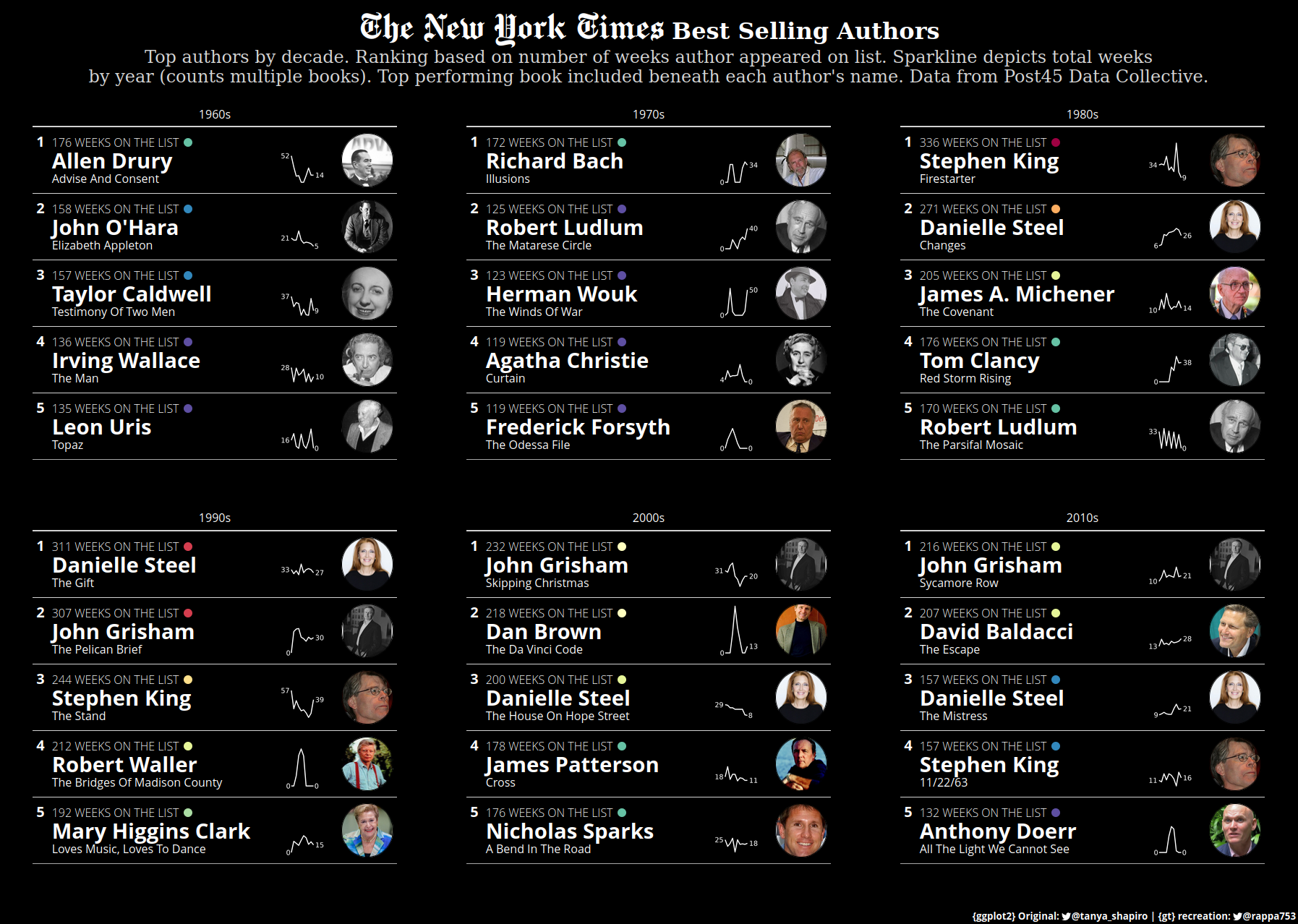
This one is a recreation of an awesome table Tanya Shapiro made with {ggplot2}. It is a huge table, so you’ll probably need to look at this on a large screen. But just to be safe. Here’s a screenshot of the table as well.
| The New York Times Best Selling Authors Top authors by decade. Ranking based on number of weeks author appeared on list. Sparkline depicts total weeks by year (counts multiple books). Top performing book included beneath each author’s name. Data from Post45 Data Collective. |
||||||||||||||
|
|
| ||||||||||||
| {ggplot2} Original: @tanya_shapiro | {gt} recreation: @rappa753 | ||||||||||||||


5.2.1 Data Preparation
The first thing we need to do is get the data. This requires a bit of data wrangling on the underlying TidyTuesdaty data set. The following code finds the top 5 authors by decade, their best book and the data for the sparkline plot.
# Book finder helper function
find_best_book <- function(decade, author) {
best_books <- nyt_dat |>
filter(decade == !!decade, author == !!author) |>
count(title, sort = TRUE)
best_books[[1, 'title']] |> str_to_title()
}
# Sparkline helper function
find_number_of_weeks_per_year <- function(decade, author){
nyt_dat |>
filter(decade == !!decade, author == !!author) |>
count(year, name = 'weeks') |>
complete(tibble(year = decade:(decade + 9)), fill = list(weeks = 0)) |>
arrange(year) |>
pull(weeks)
}
# Data from the TidyTuesday repo
nyt_dat <- readr::read_tsv('https://raw.githubusercontent.com/rfordatascience/tidytuesday/master/data/2022/2022-05-10/nyt_full.tsv') |>
mutate(decade = (year %/% 10) * 10)
# Find top 5 authors
top5_authors_by_decade <- nyt_dat |>
filter(between(year, 1960, 2019)) |>
count(author, decade, sort = T, name = 'weeks') |>
group_by(decade) |>
slice_max(weeks, n = 5) |>
ungroup()
# Find their best book and the info for the sparlines
top5_authors_and_book_by_decade <- top5_authors_by_decade |>
mutate(
best_book = map2_chr(decade, author, find_best_book),
sparkline_weeks = map2(decade, author, find_number_of_weeks_per_year)
)
top5_authors_and_book_by_decade
## # A tibble: 30 × 5
## author decade weeks best_book sparkline_weeks
## <chr> <dbl> <int> <chr> <list>
## 1 Allen Drury 1960 176 Advise And Consent <int [10]>
## 2 John O'Hara 1960 158 Elizabeth Appleton <int [10]>
## 3 Taylor Caldwell 1960 157 Testimony Of Two Men <int [10]>
## 4 Irving Wallace 1960 136 The Man <int [10]>
## 5 Leon Uris 1960 135 Topaz <int [10]>
## 6 Richard Bach 1970 172 Illusions <int [10]>
## 7 Robert Ludlum 1970 125 The Matarese Circle <int [10]>
## 8 Herman Wouk 1970 123 The Winds Of War <int [10]>
## 9 Agatha Christie 1970 119 Curtain <int [10]>
## 10 Frederick Forsyth 1970 119 The Odessa File <int [10]>
## # ℹ 20 more rowsNext, we find images of the authors online and save them in a tibble image_links. This tibble can then be joined with top5_authors_and_book_by_decade.
image_links <- tibble(
author = top5_authors_and_book_by_decade |> pull(author) |> unique(),
img = c(
'https://images.gr-assets.com/authors/1327446818p8/77616.jpg',
'https://upload.wikimedia.org/wikipedia/commons/thumb/c/c5/John_O%27Hara_cph.3b08576.jpg/1024px-John_O%27Hara_cph.3b08576.jpg',
'https://upload.wikimedia.org/wikipedia/commons/8/88/Taylor_caldwell_a.jpg',
'https://upload.wikimedia.org/wikipedia/commons/thumb/0/0c/Irving_Wallace%2C_1972.jpg/330px-Irving_Wallace%2C_1972.jpg',
'https://upload.wikimedia.org/wikipedia/commons/d/d6/Leon_Uris_%28cropped%29.jpg',
'https://images-na.ssl-images-amazon.com/images/I/41RMdx8BJHL.__01_SX120_CR0,0,120,120__.jpg',
'https://upload.wikimedia.org/wikipedia/en/a/a2/Robert_Ludlum_%281927-2001%29.jpg',
'https://upload.wikimedia.org/wikipedia/commons/thumb/4/49/Herman_Wouk_%28cropped%29.jpg/330px-Herman_Wouk_%28cropped%29.jpg',
'https://upload.wikimedia.org/wikipedia/commons/thumb/c/cf/Agatha_Christie.png/330px-Agatha_Christie.png',
'https://upload.wikimedia.org/wikipedia/commons/thumb/9/9d/Frederick_Forsyth_-_01.jpg/375px-Frederick_Forsyth_-_01.jpg',
'https://upload.wikimedia.org/wikipedia/commons/thumb/e/e3/Stephen_King%2C_Comicon.jpg/330px-Stephen_King%2C_Comicon.jpg',
'https://images1.penguinrandomhouse.com/author/29599',
'https://upload.wikimedia.org/wikipedia/commons/thumb/d/dc/James_Albert_Michener_%C2%B7_DN-SC-92-05368.JPEG/330px-James_Albert_Michener_%C2%B7_DN-SC-92-05368.JPEG',
'https://upload.wikimedia.org/wikipedia/commons/thumb/9/98/Tom_Clancy_at_Burns_Library_cropped.jpg/330px-Tom_Clancy_at_Burns_Library_cropped.jpg',
'https://upload.wikimedia.org/wikipedia/commons/thumb/5/5f/Grisham_John_by_C_Harrison_.jpg/300px-Grisham_John_by_C_Harrison_.jpg',
'https://upload.wikimedia.org/wikipedia/en/7/70/Robert_James_Waller.jpg',
'https://upload.wikimedia.org/wikipedia/commons/thumb/b/bf/Mary_Higgins_Clark_at_the_Mazza_Museum.jpg/330px-Mary_Higgins_Clark_at_the_Mazza_Museum.jpg',
'https://upload.wikimedia.org/wikipedia/commons/thumb/8/8b/Dan_Brown_bookjacket_cropped.jpg/330px-Dan_Brown_bookjacket_cropped.jpg',
'https://upload.wikimedia.org/wikipedia/commons/1/1d/James_Patterson.jpg',
'https://upload.wikimedia.org/wikipedia/commons/a/af/Nicholas-Sparks-Autograph-1-4-06.jpg',
'https://upload.wikimedia.org/wikipedia/commons/thumb/3/3d/David_Baldacci_-_2015_National_Book_Festival_%286%29.jpg/330px-David_Baldacci_-_2015_National_Book_Festival_%286%29.jpg',
'https://upload.wikimedia.org/wikipedia/commons/thumb/6/61/Anthony_Doerr_%282015%29.jpg/330px-Anthony_Doerr_%282015%29.jpg'
)
)
full_dat <- top5_authors_and_book_by_decade |>
left_join(image_links)5.2.2 Sparklines
Next, we can create the sparklines for each table entry. This requires two steps.
Find the highest number per year of how many times an author appeared in the bestseller list. This number can be higher than 52 due to multiple books. Knowing this number ensures that all of our sparklines are using the same y-axis.
Build a function that transforms the vector of weeks per year into a ggplot. Keep in mind that the sizes need to be large in the ggplot so that they are legible in the small table image later on.
# can be higher than 52 bc of multiple books
highest_week_count_per_year <- full_dat |>
pull(sparkline_weeks) |>
map_dbl(max) |>
max()
create_sparkline <- function(sparkline) {
ggplot() +
geom_line(
mapping = aes(x = seq_along(sparkline), y = sparkline),
color = 'white',
linewidth = 3
) +
annotate(
'text',
x = c(1, 10),
y = sparkline[c(1, 10)],
label = sparkline[c(1, 10)],
color = 'white',
hjust = c(1.2, -0.2),
size = 16
) +
coord_cartesian(xlim = c(-5, 15), ylim = c(0, highest_week_count_per_year)) +
theme_void() +
theme(plot.background = element_rect(fill = 'black'))
}
create_sparkline(25 * runif(10))
5.2.3 Decade table
Ok great, we have a function for sparklines now. Now, let us create the table for a singledecade. For that we will need three things.
A function that maps the number of weeks to a color (for the little colored circles)
A function that creates the HTML code for the small colored circles
A function that stacks the following information as we’ve seen in the intial table using HTML:
- number of weeks
- author name
- author’s best book
- HTML code of circle
These three functions look like this.
# Maps number of weeks to colors
map2color <- function(x, pal = rev(RColorBrewer::brewer.pal(11, 'Spectral')), limits=NULL){
if(is.null(limits)) limits <- range(x)
pal[findInterval(x,seq(limits[1],limits[2],length.out=length(pal)+1), all.inside=TRUE)]
}
# Creates colored circle which is really just a styled <span> tag
create_point_span <- function(color, size) {
glue::glue(
'<span style="height: {size}em;width: {size}em;background-color: {color};border-radius: 50%;margin-top:4px;display:inline-block;margin-left:2px;"></span>'
)
}
# Formats the author infos via styled <span> tags and line breaks <br>
format_text <- function(weeks, author, best_book, colors) {
glue::glue(
'<span style = "color:white;font-weight:lighter;font-size:12pt;">{str_to_upper(weeks)} WEEKS ON THE LIST</span> {create_point_span(colors, 0.75)}',
'<br>',
'<span style = "color:white;font-weight:bold;font-size:22pt;">{author}</span>',
'<br>',
'<span style = "color:white;font-size:12pt;">{best_book}</span>'
)
}Now we can apply these functions to get our data set ready for gt(). Here, we will use the data of the 1960s.
decade <- 1960
decade_data <- full_dat |>
# Create colors before filtering (for consistent colors across decades)
mutate(color = map2color(weeks)) |>
filter(decade == !!decade) |>
mutate(
# Shorten long names
author = if_else(
author == 'Robert James Waller',
'Robert Waller',
author
),
# Add ranking (authors are already sorted)
rank = 1:5,
# Format decade label
decade = paste0(decade, 's'),
# create stacked author info
joined_text = pmap_chr(
.l = list(weeks, author, best_book, color),
format_text
)
) |>
select(rank, decade, joined_text, sparkline_weeks, img)
decade_data
## # A tibble: 5 × 5
## rank decade joined_text sparkline_weeks img
## <int> <chr> <chr> <list> <chr>
## 1 1 1960s "<span style = \"color:white;font-weight:l… <int [10]> http…
## 2 2 1960s "<span style = \"color:white;font-weight:l… <int [10]> http…
## 3 3 1960s "<span style = \"color:white;font-weight:l… <int [10]> http…
## 4 4 1960s "<span style = \"color:white;font-weight:l… <int [10]> http…
## 5 5 1960s "<span style = \"color:white;font-weight:l… <int [10]> http…Perfect. We’re ready to pass this to gt(). Once we do that we will
- Use
decadeasgroupname_colso that the label appears on top - Turn image URLs into images
- Transform the sparkline data into plots
- Adjust widths so that the texts fit into their column and image are round
- Format the
joined_textcolumn as Markdown (so that the HTML code is rendered) - Turn background black so text is legible
img_size <- 75
# Use custom img_circles function from Chapter 2
my_gt_img_circles <- function(gt_tbl, columns, height_px) {
gt_tbl |>
gt_img_rows(columns = columns, height = 100) |>
text_transform(
locations = cells_body(columns = columns),
fn = function(x) {
css_style <- htmltools::css(
border_radius = '100%',
border = '2px solid black',
overflow = 'hidden',
height = glue::glue('{height_px}px'),
width = glue::glue('{height_px}px')
)
glue::glue(
'<div style = "{css_style}">{x}</div>'
)
}
)
}
barely_styled_decade_table <- decade_data |>
gt(groupname_col = 'decade') |>
my_gt_img_circles(column = 'img', height = img_size) |>
text_transform(
locations = cells_body(columns = sparkline_weeks),
fn = function(column) {
map(column, ~c(str_split_1(., pattern = ', '))) |>
map(parse_number) |>
map(create_sparkline) |>
# Save images manually bc ggplot_img() seems to lose some imgs
walk2(1:5, \(x, y) {
ggsave(
filename = paste0('imgs/', decade, '_', y, '.png'),
plot = x,
device = 'png',
height = 10,
width = 10,
unit = 'cm'
)
})
glue::glue(
'<img src="imgs/{decade}_{seq_along(column)}.png" style="height:75px"></img>'
)
}
) |>
cols_width(
img ~ px(82), # needs to be a little more than 75px
joined_text ~ px(300),
sparkline_weeks ~ px(100)
) |>
fmt_markdown(columns = c('joined_text')) |>
tab_options(table.background.color = 'black')
barely_styled_decade_table| rank | joined_text | sparkline_weeks | img |
|---|---|---|---|
| 1960s | |||
| 1 | 176 WEEKS ON THE LIST Allen Drury Advise And Consent |
 |
|
| 2 | 158 WEEKS ON THE LIST John O’Hara Elizabeth Appleton |
 |
|
| 3 | 157 WEEKS ON THE LIST Taylor Caldwell Testimony Of Two Men |
 |
|
| 4 | 136 WEEKS ON THE LIST Irving Wallace The Man |
 |
|
| 5 | 135 WEEKS ON THE LIST Leon Uris Topaz |
 |
|
Finally, we apply some more styling and then our decade table is good to go.
barely_styled_decade_table |>
tab_style(
style = cell_text(size = '15pt', weight = 'bold', v_align = 'top'),
locations = cells_body('rank')
) |>
tab_style(
locations = cells_row_groups(),
style = cell_text(align = 'center')
) |>
tab_options(
table.background.color = 'black',
table.font.color = 'white',
table.font.names = 'Open Sans',
column_labels.hidden = TRUE,
row_group.border.top.style = 'none',
row_group.border.bottom.style = 'none',
table.border.bottom.style = 'solid',
table.border.bottom.width = px(1),
table.border.top.style = 'none',
table_body.border.bottom.style = 'none',
table_body.border.top.style = 'none',
heading.border.bottom.style = 'none',
column_labels.border.top.style = 'none',
) | 1960s | |||
|---|---|---|---|
| 1 | 176 WEEKS ON THE LIST Allen Drury Advise And Consent |
|
|
| 2 | 158 WEEKS ON THE LIST John O’Hara Elizabeth Appleton |
|
|
| 3 | 157 WEEKS ON THE LIST Taylor Caldwell Testimony Of Two Men |
|
|
| 4 | 136 WEEKS ON THE LIST Irving Wallace The Man |
|
|
| 5 | 135 WEEKS ON THE LIST Leon Uris Topaz |
|
|
Now we know how to create one decade table. Time to wrap the logic into a function. We’ll call it create_decade_table(). Very original, I know.
Code
create_decade_table <- function(decade, img_size = 75) {
decade_data <- full_dat |>
# Create colors before filtering (for consistent colors across decades)
mutate(color = map2color(weeks)) |>
filter(decade == !!decade) |>
mutate(
# Shorten long names
author = if_else(
author == 'Robert James Waller',
'Robert Waller',
author
),
# Add ranking (authors are already sorted)
rank = 1:5,
# Format decade label
decade = paste0(decade, 's'),
# create stacked author info
joined_text = pmap_chr(
.l = list(weeks, author, best_book, color),
format_text
)
) |>
select(rank, decade, joined_text, sparkline_weeks, img)
barely_styled_decade_table <- decade_data |>
gt(groupname_col = 'decade') |>
my_gt_img_circles(column = 'img', height = img_size) |>
text_transform(
locations = cells_body(columns = sparkline_weeks),
fn = function(column) {
map(column, ~c(str_split_1(., pattern = ', '))) |>
map(parse_number) |>
map(create_sparkline) |>
# Save images manually bc ggplot_img() seems to lose some imgs
walk2(1:5, \(x, y) {
ggsave(
filename = paste0('imgs/', decade, '_', y, '.png'),
plot = x,
device = 'png',
height = 10,
width = 10,
unit = 'cm'
)
})
glue::glue(
'<img src="imgs/{decade}_{seq_along(column)}.png" style="height:75px"></img>'
)
}
) |>
cols_width(
img ~ px(82), # needs to be a little more than 75px
joined_text ~ px(300),
sparkline_weeks ~ px(100)
) |>
fmt_markdown(columns = c('joined_text')) |>
tab_options(table.background.color = 'black')
barely_styled_decade_table |>
tab_style(
style = cell_text(size = '15pt', weight = 'bold', v_align = 'top'),
locations = cells_body('rank')
) |>
tab_style(
locations = cells_row_groups(),
style = cell_text(align = 'center')
) |>
tab_options(
table.background.color = 'black',
table.font.color = 'white',
table.font.names = 'Open Sans',
column_labels.hidden = TRUE,
row_group.border.top.style = 'none',
row_group.border.bottom.style = 'none',
table.border.bottom.style = 'solid',
table.border.bottom.width = px(1),
table.border.top.style = 'none',
table_body.border.bottom.style = 'none',
table_body.border.top.style = 'none',
heading.border.bottom.style = 'none',
column_labels.border.top.style = 'none',
)
}create_decade_table(1960)| 1960s | |||
|---|---|---|---|
| 1 | 176 WEEKS ON THE LIST Allen Drury Advise And Consent |
|
|
| 2 | 158 WEEKS ON THE LIST John O’Hara Elizabeth Appleton |
|
|
| 3 | 157 WEEKS ON THE LIST Taylor Caldwell Testimony Of Two Men |
|
|
| 4 | 136 WEEKS ON THE LIST Irving Wallace The Man |
|
|
| 5 | 135 WEEKS ON THE LIST Leon Uris Topaz |
|
|
create_decade_table(1970)| 1970s | |||
|---|---|---|---|
| 1 | 172 WEEKS ON THE LIST Richard Bach Illusions |
 |
|
| 2 | 125 WEEKS ON THE LIST Robert Ludlum The Matarese Circle |
 |
|
| 3 | 123 WEEKS ON THE LIST Herman Wouk The Winds Of War |
 |
|
| 4 | 119 WEEKS ON THE LIST Agatha Christie Curtain |
 |
|
| 5 | 119 WEEKS ON THE LIST Frederick Forsyth The Odessa File |
 |
|
create_decade_table(1980)| 1980s | |||
|---|---|---|---|
| 1 | 336 WEEKS ON THE LIST Stephen King Firestarter |
 |
|
| 2 | 271 WEEKS ON THE LIST Danielle Steel Changes |
 |
|
| 3 | 205 WEEKS ON THE LIST James A. Michener The Covenant |
 |
|
| 4 | 176 WEEKS ON THE LIST Tom Clancy Red Storm Rising |
 |
|
| 5 | 170 WEEKS ON THE LIST Robert Ludlum The Parsifal Mosaic |
 |
|
create_decade_table(1990)| 1990s | |||
|---|---|---|---|
| 1 | 311 WEEKS ON THE LIST Danielle Steel The Gift |
 |
|
| 2 | 307 WEEKS ON THE LIST John Grisham The Pelican Brief |
 |
|
| 3 | 244 WEEKS ON THE LIST Stephen King The Stand |
 |
|
| 4 | 212 WEEKS ON THE LIST Robert Waller The Bridges Of Madison County |
 |
|
| 5 | 192 WEEKS ON THE LIST Mary Higgins Clark Loves Music, Loves To Dance |
 |
|
create_decade_table(2000)| 2000s | |||
|---|---|---|---|
| 1 | 232 WEEKS ON THE LIST John Grisham Skipping Christmas |
 |
|
| 2 | 218 WEEKS ON THE LIST Dan Brown The Da Vinci Code |
 |
|
| 3 | 200 WEEKS ON THE LIST Danielle Steel The House On Hope Street |
 |
|
| 4 | 178 WEEKS ON THE LIST James Patterson Cross |
 |
|
| 5 | 176 WEEKS ON THE LIST Nicholas Sparks A Bend In The Road |
 |
|
create_decade_table(2010)| 2010s | |||
|---|---|---|---|
| 1 | 216 WEEKS ON THE LIST John Grisham Sycamore Row |
 |
|
| 2 | 207 WEEKS ON THE LIST David Baldacci The Escape |
 |
|
| 3 | 157 WEEKS ON THE LIST Danielle Steel The Mistress |
 |
|
| 4 | 157 WEEKS ON THE LIST Stephen King 11/22/63 |
 |
|
| 5 | 132 WEEKS ON THE LIST Anthony Doerr All The Light We Cannot See |
 |
|
5.2.4 Assembling the table
With some functional programming we can collect the HTML code for all tables in one tibble. Then, we can assemble a custom HTML text for the table and create our first table prototype.
# Create tables for each decade and convert them to HTML
raw_tables <- map(seq(1960, 2010, 10), create_decade_table) |>
map_chr(as_raw_html)
ordered_tibble <- tibble(
col1 = raw_tables[c(1, 4)],
col2 = raw_tables[c(2, 5)],
col3 = raw_tables[c(3, 6)]
)
## Create custom HTML text for title to use many different styles
title <- paste0(
"<span style='font-family:Chomsky;font-size:42pt;color:white;'> The New York Times</span>",
"<span style='font-family:opensans;font-size:24pt;color:white;'> **Best Selling Authors**</span>",
"<br><span style='font-family:opensans;font-size:18pt;color:#D6D6D6'>Top authors by decade. Ranking based on number of weeks author appeared on list. Sparkline depicts total weeks<br>by year (counts multiple books). Top performing book included beneath each author's name. Data from Post45 Data Collective.</span><br>"
)
ordered_tibble |>
gt(id = 'bestseller_collected') |>
fmt_markdown(columns = everything()) |>
tab_header(title = md(title)) |>
tab_footnote(
html(glue::glue(
'{ggplot2} Original: <<fontawesome::fa("twitter")>>@tanya_shapiro |
{gt} recreation: <<fontawesome::fa("twitter")>>@rappa753',
.open = "<<", .close = ">>"
))
) |>
cols_width(
col1 ~ px(600),
col2 ~ px(600),
col3 ~ px(600)
) |>
tab_style(
locations = cells_body(rows = 1),
style = cell_borders(style = 'hidden')
) |>
tab_options(table.background.color = 'black')| The New York Times Best Selling Authors Top authors by decade. Ranking based on number of weeks author appeared on list. Sparkline depicts total weeks by year (counts multiple books). Top performing book included beneath each author’s name. Data from Post45 Data Collective. |
||||||||||||||
| col1 | col2 | col3 | ||||||||||||
|---|---|---|---|---|---|---|---|---|---|---|---|---|---|---|
|
|
| ||||||||||||
| {ggplot2} Original: @tanya_shapiro | {gt} recreation: @rappa753 | ||||||||||||||


Of course we still have some styling to do. So let’s finish off with this.
ordered_tibble |>
gt(id = 'bestseller_collected_styled') |>
fmt_markdown(columns = everything()) |>
tab_header(title = md(title)) |>
tab_footnote(
html(glue::glue(
'{ggplot2} Original: <<fontawesome::fa("twitter")>>@tanya_shapiro |
{gt} recreation: <<fontawesome::fa("twitter")>>@rappa753',
.open = "<<", .close = ">>"
))
) |>
cols_width(
col1 ~ px(600),
col2 ~ px(600),
col3 ~ px(600)
) |>
tab_style(
locations = cells_body(rows = 1),
style = cell_borders(style = 'hidden')
) |>
tab_options(table.background.color = 'black') |>
tab_style(
locations = cells_body(rows = 1),
style = cell_borders(style = 'hidden')
) |>
tab_options(
table.background.color = 'black',
column_labels.hidden = TRUE,
table_body.border.bottom.style = 'none',
) |>
opt_css(
'#bestseller_collected_styled .gt_footnote {
text-align: right;
padding-top: 20px;
padding-bottom:5px;
font-family:"Open Sans";
font-size:10pt;
font-weight:bold;
}
#bestseller_collected_styled .gt_row {
border-top-color: grey;
border-bottom-color: grey;
}
#bestseller_collected_styled thead, tbody, tfoot, tr, td, th {
border-color: inherit;
border-style: solid;
border-width: 0;
}
#bestseller_collected_styled thead, tbody, tfoot, tr, td, th {
border-color: inherit;
border-style: solid;
border-width: 0;
}
div#bestseller_collected_styled {line-height:1.1;}
'
) | The New York Times Best Selling Authors Top authors by decade. Ranking based on number of weeks author appeared on list. Sparkline depicts total weeks by year (counts multiple books). Top performing book included beneath each author’s name. Data from Post45 Data Collective. |
||||||||||||||
|
|
| ||||||||||||
| {ggplot2} Original: @tanya_shapiro | {gt} recreation: @rappa753 | ||||||||||||||
5.3 LaTeX formulas
Let’s do one more little case study. This one does not require any custom styling. In the absence of support for formulas with MathJax, this is a workaround of incorporating formulas in your tables. It probably won’t work on exports to PDF but for HTML outputs it should do.
The trick we’re going to use is as follows.
Pass LaTeX formulas to
tex2image()from{exams}. This will transform your formula into an svg image and save it to a file.Read that file and change the colors to whatever you like via text replacement using
str_replace_all(). By default all elements are black.
exams::tex2image(
'$\\overline{X_n} = \\sum\\limits_{k = 1}^{n} x_k $',
format = 'svg',
dir = here::here(),
name = 'formula'
)
svg_formula_black <- read_lines('formula.svg') |>
str_flatten()
svg_formula_white <- svg_formula_black |>
# Overline color uses stroke, rest uses fill
str_replace_all('stroke:rgb\\(0%,0%,0%\\)', 'stroke:#FFFFFF') |>
str_replace_all('fill:rgb\\(0%,0%,0%\\)', 'fill:#FFFFFF')
tibble(char = svg_formula_black, char2 = 'bla') |>
gt() |>
opt_stylize(style = 3) |>
tab_spanner(
label = md(svg_formula_white),
columns = 1:2
) |>
fmt_markdown(columns = 'char') |>
tab_header(title = 'This is a table with formulas as svgs')| This is a table with formulas as svgs | |
|
|
|
|---|---|
| char | char2 |
| bla | |
Now let’s use a second formula in the table. The idea is basically the same. But you have to be careful for one very small reason.
The svg code for the formula images that we get from tex2image() always contains IDs that start with glyph. But all IDs need to be unique. Hence, the second svg code that we generate with tex2image() cannot use glyph for its IDs. Text replacement solves this issue.
exams::tex2image(
'$\\int_0^\\infty f(x) dx$',
format = 'svg',
dir = here::here(),
name = 'second_formula'
)
svg_formula_black_integral <- readLines('formula2.svg') |>
str_flatten() |>
str_replace_all('glyph', 'some_other_id')
tibble(char = svg_formula_black, char2 = svg_formula_black_integral) |>
gt() |>
opt_stylize(style = 3) |>
tab_spanner(
label = md(svg_formula_white),
columns = 1:2
) |>
fmt_markdown(columns = c('char', 'char2')) |>
tab_header(title = 'This is a table with formulas as svgs')| This is a table with formulas as svgs | |
|
|
|
|---|---|
| char | char2 |
5.4 Summary
Alright, alright, alright. What a ride.1 I hope this chapter showed you how everything we’ve learned in this book can be put together to create a range of cool tables.
You probably want to share your tables with the world. Sharing them in Quarto documents can be one way to do that. But there’s one thing you have to watch out for. Next stop: Quarto.
Maybe I’m just a little bit dramatic.↩︎